DeepSeek V4: Towards Highly Efficient Million-Token Context Intelligence
Link:
- Technical Report: DeepSeek_V4.pdf
- Hugging Face Model Card: deepseek-ai/DeepSeek-V4-Pro
- Official Inference Code: inference/model.py
- Transformers Code: modeling_deepseek_v4.py
- Transformers Docs: DeepSeek-V4
[toc]
Main Contributions
- 1M Context: DeepSeek-V4 系列把上下文长度推到 1M tokens。重点不是单纯把 RoPE 拉长,而是围绕长上下文重新设计 attention、KV cache 和 sparse selection。
- Hybrid Attention Architecture: 使用 Compressed Sparse Attention (CSA) 和 Heavily Compressed Attention (HCA) 混合结构,把近邻 token 精确保留,把远程 token 压缩后选择性读取。
- Manifold-Constrained Hyper-Connections (mHC): 把传统 residual stream 扩成多条 hidden streams,并用受约束的 mixing 矩阵进行合并与传播。
- MoE Routing Update: MoE router 支持
sqrt softplus分数函数和前若干层的 hash routing。 - MTP: 继续使用 Multi-Token Prediction 思路,为训练提供 next-n token 信号,也为后续推理辅助留下结构入口。
- Training / Post-training: 官方模型卡中提到 32T+ tokens 预训练、Muon optimizer,以及 SFT + GRPO + on-policy distillation 的后训练路线。
官方给出的模型规模如下:
| Model | Total Params | Activated Params | Context Length | Precision |
|---|---|---|---|---|
| DeepSeek-V4-Flash | 284B | 13B | 1M | FP4 + FP8 mixed |
| DeepSeek-V4-Pro | 1.6T | 49B | 1M | FP4 + FP8 mixed |
| DeepSeek-V4-Flash-Base | 284B | 13B | 1M | FP8 mixed |
| DeepSeek-V4-Pro-Base | 1.6T | 49B | 1M | FP8 mixed |
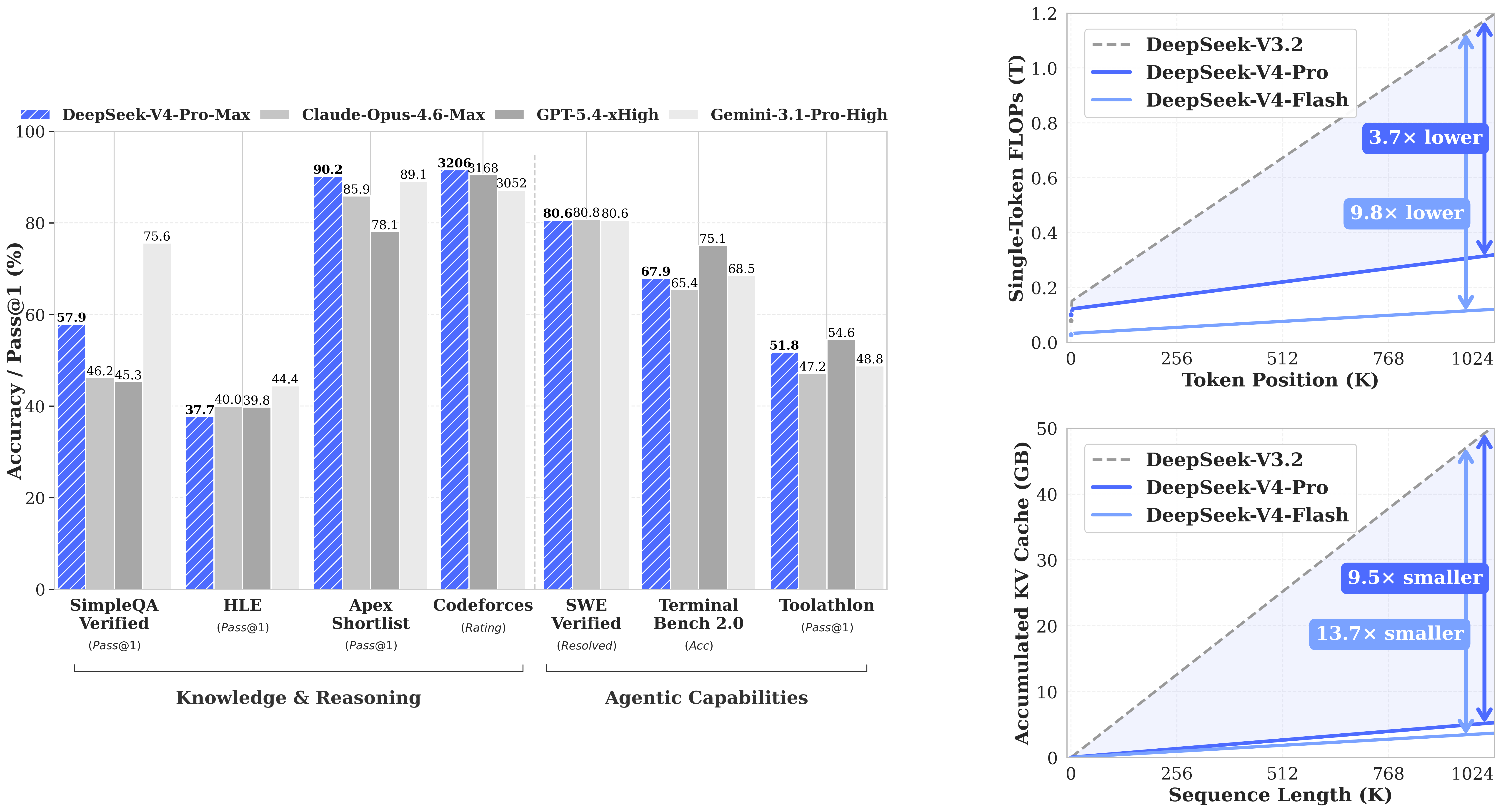
1. 整体架构
我先把 DeepSeek-V4 看成三条线:
- Attention 线: 用 sliding window 处理最近 token,用 CSA / HCA 处理远程 token。
- Residual 线: 用 mHC 替代简单 residual,让 hidden state 在多条 stream 之间混合。
- MoE 线: 继续走 sparse MoE,但 router 分数和部分层路由方式有变化。
一个比较接近源码的 block 级流程如下:
flowchart TD
    A[input_ids] --> B[Token Embedding]
    B --> C[Expand to n_hc streams]
    C --> D[mHC pre mix for attention]
    D --> E[RMSNorm]
    E --> F[Hybrid Attention: SWA + CSA/HCA]
    F --> G[mHC post mix]
    G --> H[mHC pre mix for MoE]
    H --> I[RMSNorm]
    I --> J[MoE FFN: hash/top-k router + experts]
    J --> K[mHC post mix]
    K --> L[Hyper Head + RMSNorm + LM Head]
在官方 inference 代码里,这个结构大概对应:
Transformer: embedding、主干 blocks、lm head、MTP blocks。Block: attention + MoE,两处都包了一层 hyper-connection。Attention: sliding window cache + optional compressor + optional indexer。MoE: router、routed experts、shared expert。
需要注意:Transformers 版本为了兼容 generate、cache 和 HF API,类名更细;官方 inference 版本更像“论文结构的最小可读实现”。这篇笔记会同时参考两者,但讲概念时优先贴近官方 inference 写法。
2. 和 DeepSeek-V3 / V3.2 的关系
DeepSeek-V3 的两个核心词是 MLA 和 DeepSeekMoE。V4 没有丢掉 MoE 路线,但长上下文这件事变成了中心问题。
可以先这样理解:
| 模型 | 主要 attention / cache 思路 | MoE | 长上下文处理重点 |
|---|---|---|---|
| DeepSeek-V2 | MLA 降低 KV cache | DeepSeekMoE | 经济型推理 |
| DeepSeek-V3 | MLA + MTP + MoE 训练优化 | DeepSeekMoE | 训练效率和推理能力 |
| DeepSeek-V4 | CSA + HCA hybrid attention | MoE + hash/top-k router | 1M context 下压缩和稀疏选择 |
V4 的关键不是“把所有历史 token 都完整记下来”。如果 1M tokens 全量 KV cache 直接进 attention,显存和算力都不现实。V4 的路线是:
- 最近窗口:保留完整 KV,保证局部上下文精度。
- 更远上下文:压缩成少量 compressed entries。
- 需要读远程信息时:用 indexer 从 compressed entries 里选 top-k。
所以 V4 的 attention 更像一个分层记忆系统:近处看原文,远处看摘要,必要时再从摘要索引里挑重点。
3. MTP: Multi-Token Prediction
3.1 MTP 是什么
MTP = Multi-Token Prediction。
普通 causal LM 的训练目标是:
\[p(x_{t+1}\mid x_{\le t})\]也就是每个位置只预测下一个 token。MTP 的思路是:在主 next-token loss 之外,再让模型预测更远的 token,例如:
\[p(x_{t+2}\mid x_{\le t}),\quad p(x_{t+3}\mid x_{\le t}),\quad \ldots\]可以写成一个简化目标:
\[\mathcal{L}_{\mathrm{MTP}} = \frac{1}{D}\sum_{k=1}^{D} \mathrm{CE}\big(p_k(x_{t+k}\mid x_{\le t}), x_{t+k}\big)\]其中 $D$ 是额外预测的步数。
直觉上,next-token prediction 只要求模型把眼前一步做好;MTP 会逼模型在 hidden state 里保留更多“接下来几步可能怎么走”的信息。DeepSeek-V3 技术报告里已经使用过 MTP,V4 继续保留了这个方向。
3.2 DeepSeek-V4 里的 MTPBlock
官方 inference 代码里有 n_mtp_layers 和 MTPBlock。从结构上看,MTPBlock 会拿两类信息:
- 当前主干模型的 hidden state。
- shifted input token 的 embedding。
先对齐源码接口。官方 inference 里的 MTPBlock.forward 是:
def forward(self, x, start_pos, input_ids):
    e = self.embed(input_ids)
    e = self.enorm(e)
    x = self.hnorm(x)
    x = self.e_proj(e).unsqueeze(2) + self.h_proj(x)
    x = super().forward(x, start_pos, input_ids)
    logits = self.head(x, self.hc_head_fn, self.hc_head_scale, self.hc_head_base, self.norm)
    return logits
也就是说,源码里的 MTPBlock 不会自己构造 shifted tokens。它只要求调用方传入一段 input_ids,然后把这段 token 的 embedding 和上一层 hidden streams 融合。真正的 shift 逻辑属于训练数据/调用逻辑:第 1 个 MTPBlock 传入 x[t+1],目标是 x[t+2];第 2 个 MTPBlock 再传入 x[t+2],目标是 x[t+3]。
这里的 shifted input token 指的是“向后错位后的真实 token”。假设原始序列是:
x0, x1, x2, x3, x4, x5
普通 next-token prediction 在位置 t=2 使用 x0, x1, x2 的上下文预测 x3。
MTP 想继续预测更远的位置。为了预测 x4,MTPBlock 会额外看到一个 shifted token,也就是 x3 的 embedding。这里不是把 x3 当成模型生成结果,而是在训练时把真实序列右移后喂给 MTP 模块,帮助它构造“预测下一步的下一步”的中间状态。
可以把它想成:
| 位置 | 主模型看到的上下文 | 主 LM head 目标 | 第 1 个 MTPBlock 额外输入 | 第 1 个 MTPBlock 目标 |
|---|---|---|---|---|
t=0 |
x0 |
x1 |
x1 |
x2 |
t=1 |
x0, x1 |
x2 |
x2 |
x3 |
t=2 |
x0, x1, x2 |
x3 |
x3 |
x4 |
所以 shifted_input_ids 不是一个新 token,也不是预测 token,而是训练数据中已经存在的 token,只是相对当前位置向后平移了一格。如果有多个 MTP 层,第 2 个 MTPBlock 会继续用更后面的 shifted token,去预测更远的目标。
然后 MTPBlock 会把 shifted token embedding 和主 hidden state 分别投影、相加,再过一个 block,最后接同一个 head 输出 logits。
用等价伪代码表示:
tokens = [x0, x1, x2, x3, x4, x5]
T = len(tokens)

# 主模型:位置 t 的 hidden 用来预测 x[t+1]
# 有效位置:t = 0, 1, 2, 3, 4
main_hidden = backbone(tokens[:-1])
main_logits = lm_head(main_hidden)
main_loss = 0
for t in range(T - 1):
    main_loss += CE(main_logits[t], tokens[t + 1])

# 第 1 个 MTPBlock:额外输入 tokens[t+1],目标变成 tokens[t+2]
# 有效位置:t = 0, 1, 2, 3
shifted_1 = tokens[1:]               # x1, x2, x3, x4, x5
target_1 = tokens[2:]                # x2, x3, x4, x5
mtp_hidden_1 = mtp_block_1(main_hidden[:-1], shifted_1[:-1])
mtp_logits_1 = lm_head(mtp_hidden_1)
mtp_loss_1 = 0
for t in range(T - 2):
    mtp_loss_1 += CE(mtp_logits_1[t], target_1[t])

# 如果有第 2 个 MTPBlock:继续往后错一格,目标变成 tokens[t+3]
# 有效位置:t = 0, 1, 2
shifted_2 = tokens[2:]               # x2, x3, x4, x5
target_2 = tokens[3:]                # x3, x4, x5
mtp_hidden_2 = mtp_block_2(mtp_hidden_1[:-1], shifted_2[:-1])
mtp_logits_2 = lm_head(mtp_hidden_2)
mtp_loss_2 = 0
for t in range(T - 3):
    mtp_loss_2 += CE(mtp_logits_2[t], target_2[t])
再把一个 MTPBlock 本身展开看,它内部大概是:
class MTPBlock:
    def forward(prev_hidden_streams, shifted_input_ids):
        shifted_emb = embed(shifted_input_ids)
        token_part = e_proj(norm_embed(shifted_emb))
        hidden_part = h_proj(norm_hidden(prev_hidden_streams))

        mtp_hidden = token_part[:, :, None, :] + hidden_part
        mtp_hidden = transformer_block(mtp_hidden, shifted_input_ids)

        logits = shared_lm_head(hyper_head(mtp_hidden))
        return logits
这里有一个容易混淆的点:MTP 不是把模型一次 forward 变成“直接吐多个 token”。在公开 inference 代码里,主 Transformer.forward 默认仍然返回 next-token logits;MTPBlock 更像是额外结构,让 hidden state 多承担几个未来 token 的预测任务。
4. MoE Router、Softplus 和 Hash Route
4.1 Softplus 是什么
Softplus 的定义是:
\[\mathrm{softplus}(x)=\log(1+e^x)\]它可以看成 ReLU 的平滑版本:
\[\mathrm{ReLU}(x)=\max(0,x)\]区别是:
- ReLU 在 $x<0$ 时直接变成 0。
- Softplus 始终大于 0,并且在 0 附近是平滑的。
这对 router 分数有用,因为 MoE router 最后要得到非负权重。如果使用 softplus,负 logits 不会被硬切成 0,而是保留一个很小的正值。
4.2 Hash Route 是什么
普通 top-k router 是:
indices = topk(scores, k)
Hash route 则是:
indices = tid2eid[input_ids]
也就是说,某些层的 expert 选择不再由当前 hidden state 动态决定,而是由 token id 查表得到。
这像是把“这个 token 去哪些专家”提前写进一个表里。对应到源码,hash layer 会有一个 tid2eid 参数,它的形状大致是:
4.3 为什么要 Hash Route
这部分论文和源码能确认的是:DeepSeek-V4 确实支持前若干层使用 hash routing。至于动机,我的理解要稍微保守一点:
- 早期层的 token 表示还比较接近 token identity,用 token id 路由有一定合理性。
- hash routing 可以减少动态 top-k 路由带来的计算和通信波动。
- 固定路由可能让早期 expert 分配更稳定,降低某些 batch 下的 routing collapse 风险。
- 但它也会牺牲一部分上下文自适应能力,所以不适合所有层都这么做。
因此我会把 Hash Route 理解成:早期层用更便宜、更稳定的 token-id 路由,后续层再交给 hidden-state-based top-k router。
4.4 Hugging Face Router 代码
Hugging Face / 官方 inference 的 router 可以按这两步读:先算 routing scores,再决定 selected experts。Hash route 改的是 selected experts 的来源,不是把 expert weights 全部变成常数。
logits = linear(hidden_states, router_weight)
scores = sqrt(softplus(logits))

if hash_routing:
    selected_experts = tid2eid[input_ids]
else:
    selected_experts = topk(scores + correction_bias, k)

router_weights = gather(scores, selected_experts)
router_weights = router_weights / router_weights.sum(dim=-1, keepdim=True)
这里 correction_bias 可以影响 top-k 选择,但真正的 router_weights 仍然来自未加 bias 的 scores。也就是说,selection 和 weighting 可以使用略不同的信号。
5. mHC: Manifold-Constrained Hyper-Connections
论文第 2.2 节的写法是:先介绍 Standard Hyper-Connections (HC),再说明 mHC 相比 HC 多了哪些稳定性约束。这里我也按论文顺序记。
5.1 Standard Hyper-Connections
标准 HC 的第一步是把 residual stream 的“宽度”扩成 $n_{\mathrm{hc}}$ 条。论文里说的是:
\[\mathbb{R}^{d}\rightarrow\mathbb{R}^{n_{\mathrm{hc}}\times d}\]其中 $d$ 是真实喂给 Transformer layer 的 hidden size,$n_{\mathrm{hc}}$ 是 Hyper-Connection 的 stream 数量。Hugging Face 配置里对应字段叫 hc_mult,DeepSeek-V4 常见设置是:
hc_mult = 4
对第 $l$ 层之前的 residual state,论文定义:
\[\begin{aligned} X_l &= \left[ x_{l,1}; \ldots; x_{l,n_{\mathrm{hc}}} \right]^T &\in \mathbb{R}^{n_{\mathrm{hc}}\times d} \end{aligned}\]这里每个 $x_{l,i}\in\mathbb{R}^{d}$。所以它不是把 $d$ 切成 $d/n_{\mathrm{hc}}$,而是维护 $n_{\mathrm{hc}}$ 条完整的 $d$ 维 residual streams。
HC 引入三个线性映射:
\[A_l\in\mathbb{R}^{1\times n_{\mathrm{hc}}}\] \[B_l\in\mathbb{R}^{n_{\mathrm{hc}}\times n_{\mathrm{hc}}}\] \[C_l\in\mathbb{R}^{n_{\mathrm{hc}}\times 1}\]更新公式是论文的式 (1):
\[\begin{aligned} X_{l+1} &= B_lX_l+C_lF_l(A_lX_l) \end{aligned}\]逐项看维度:
- $A_lX_l\in\mathbb{R}^{1\times d}$:把 $n_{\mathrm{hc}}$ 条 stream collapse 成一条,作为 layer input。
- $F_l(A_lX_l)\in\mathbb{R}^{1\times d}$:第 $l$ 个实际 layer 的输出,仍然是 $d$ 维。
- $C_lF_l(A_lX_l)\in\mathbb{R}^{n_{\mathrm{hc}}\times d}$:把 layer 输出写回 $n_{\mathrm{hc}}$ 条 stream。
- $B_lX_l\in\mathbb{R}^{n_{\mathrm{hc}}\times d}$:旧 residual streams 之间的线性混合。
所以 HC 的关键点是:inner layer 仍然只处理 $d$ 维输入输出,额外扩展的是 residual stream 的宽度。 这给模型增加了一条不同于 hidden size 的扩展轴,但因为 $n_{\mathrm{hc}}$ 通常很小,所以开销相对可控。
5.2 mHC 相比 HC 改了什么
论文说标准 HC 在多层堆叠时可能出现 numerical instability。mHC 的核心改动是:不再让 $B_l$ 成为任意矩阵,而是把 $B_l$ 约束到 doubly stochastic matrices 的流形上。
论文定义的流形是 Birkhoff polytope:
\[\begin{aligned} \mathcal{M} &= \Bigl\{ M\in\mathbb{R}^{n_{\mathrm{hc}}\times n_{\mathrm{hc}}} \ \Big| M\mathbf{1}_{n_{\mathrm{hc}}}=\mathbf{1}_{n_{\mathrm{hc}}}, \ \mathbf{1}_{n_{\mathrm{hc}}}^{\top}M=\mathbf{1}_{n_{\mathrm{hc}}}^{\top}, \ M\ge 0 \Bigr\} \end{aligned}\]然后约束:
\[B_l\in\mathcal{M}\]这里的含义很具体:
- $M\mathbf{1}=\mathbf{1}$:每一行和为 1。
- $\mathbf{1}^{T}M=\mathbf{1}^{T}$:每一列和为 1。
- $M\ge 0$:所有元素非负。
论文给出的理由是:这个约束会让 $\lVert B_l\rVert_2$ 被 1 bound 住,因此 residual transformation 是 non-expansive 的。换句话说,$B_l$ 混合多条 stream 时不会无限放大信号。并且 $\mathcal{M}$ 对矩阵乘法封闭,所以多层堆叠时仍然能保持稳定性。
此外,论文还约束 $A_l$ 和 $C_l$ 非负且有界,避免不同 stream 之间因为符号相反而发生 signal cancellation。
5.3 Dynamic Parameterization
mHC 里的 $A_l,B_l,C_l$ 不是固定参数,而是动态生成的。论文把它们分成:
- dynamic component:由当前输入 $X_l$ 生成。
- static component:输入无关的可学习 bias。
给定:
\[X_l\in\mathbb{R}^{n_{\mathrm{hc}}\times d}\]先 flatten 并 RMSNorm:
\[\begin{aligned} \hat{X}_l &= \mathrm{RMSNorm}(\mathrm{vec}(X_l)) \\ &\in \mathbb{R}^{1\times n_{\mathrm{hc}}d} \end{aligned}\]然后生成 unconstrained raw parameters:
\[\begin{aligned} \tilde{A}_l &= \alpha_l^{\mathrm{pre}} \cdot (\hat{X}_lW_l^{\mathrm{pre}}) + S_l^{\mathrm{pre}} \end{aligned}\] \[\begin{aligned} \tilde{B}_l &= \alpha_l^{\mathrm{res}} \cdot \mathrm{Mat}(\hat{X}_lW_l^{\mathrm{res}}) + S_l^{\mathrm{res}} \end{aligned}\] \[\begin{aligned} \tilde{C}_l &= \alpha_l^{\mathrm{post}} \cdot (\hat{X}_lW_l^{\mathrm{post}})^T + S_l^{\mathrm{post}} \end{aligned}\]对应维度是:
\[\begin{aligned} W_l^{\mathrm{pre}},W_l^{\mathrm{post}} &\in \mathbb{R}^{n_{\mathrm{hc}}d\times n_{\mathrm{hc}}} \end{aligned}\] \[\begin{aligned} W_l^{\mathrm{res}} &\in \mathbb{R}^{n_{\mathrm{hc}}d\times n_{\mathrm{hc}}^2} \end{aligned}\] \[S_l^{\mathrm{pre}}\in\mathbb{R}^{1\times n_{\mathrm{hc}}}, \quad S_l^{\mathrm{res}}\in\mathbb{R}^{n_{\mathrm{hc}}\times n_{\mathrm{hc}}}, \quad S_l^{\mathrm{post}}\in\mathbb{R}^{n_{\mathrm{hc}}\times 1}\]其中 $\mathrm{Mat}(\cdot)$ 把 $1\times n_{\mathrm{hc}}^2$ 的向量 reshape 成 $n_{\mathrm{hc}}\times n_{\mathrm{hc}}$ 矩阵。$\alpha_l^{\mathrm{pre}},\alpha_l^{\mathrm{res}},\alpha_l^{\mathrm{post}}\in\mathbb{R}$ 是可学习 gating factors,论文说它们初始化为较小值。这样做的直觉是:训练初期更接近 static component,等训练稳定后再逐步放大 input-dependent dynamic component。
5.4 Applying Parameter Constraints
得到 raw parameters 之后,mHC 才施加约束。
对 input mapping 和 output mapping:
\[A_l=\sigma(\tilde{A}_l)\] \[C_l=2\sigma(\tilde{C}_l)\]这里 $A_l$ 的范围是 $(0,1)$,$C_l$ 的范围是 $(0,2)$。它们都是非负且有界的。
对 residual mapping,先保证正数:
\[M^{(0)}=\exp(\tilde{B}_l)\]然后用 Sinkhorn-Knopp 反复做列归一化和行归一化:
\[\begin{aligned} M^{(t)} &= T_r\left(T_c\left(M^{(t-1)}\right)\right) \end{aligned}\]其中 $T_c$ 表示 column normalization,$T_r$ 表示 row normalization。最终:
\[B_l=M^{(t_{\max})}\]论文中取:
\[t_{\max}=20\]这回答了之前那个疑问:20 次 Sinkhorn 发生在 $n_{\mathrm{hc}}\times n_{\mathrm{hc}}$ 的小矩阵上。DeepSeek-V4 常见 $n_{\mathrm{hc}}=4$,所以每个 token 的 $B_l$ 是 $4\times4$,不是 $d\times d$,也不是 $(n_{\mathrm{hc}}d)\times(n_{\mathrm{hc}}d)$。
5.5 和 Hugging Face 变量的对应
HF Transformers 里的 DeepseekV4DecoderLayer 有两个 hyper-connection 模块:
attn_hc:包住 self-attention。ffn_hc:包住 MoE / FFN。
调用形式可以概括为:
post, comb, collapsed = self.attn_hc(hidden_states)
对应论文符号:
| HF 变量 | 论文符号 | 维度 | 作用 |
|---|---|---|---|
hidden_states |
$X_l$ | $[B_{\mathrm{sz}},S,n_{\mathrm{hc}},d]$ | 多条 residual streams |
pre |
$A_l$ | $[B_{\mathrm{sz}},S,1,n_{\mathrm{hc}}]$ 或 broadcast 等价形态 | input mapping |
collapsed |
$A_lX_l$ | $[B_{\mathrm{sz}},S,d]$ | 真正喂给 attention / FFN 的输入 |
comb |
$B_l$ | $[B_{\mathrm{sz}},S,n_{\mathrm{hc}},n_{\mathrm{hc}}]$ | constrained residual mapping |
post |
$C_l$ | $[B_{\mathrm{sz}},S,n_{\mathrm{hc}},1]$ 或 broadcast 等价形态 | output mapping |
pre 没有返回,是因为它已经在 collapsed = A_lX_l 这一步用掉了。decoder layer 拿到 collapsed 后调用 attention / FFN,再把输出写回:
post, comb, collapsed = attn_hc(hidden_states)
attn_output = self_attn(norm(collapsed))
hidden_states = post[..., None] * attn_output[..., None, :] + comb @ hidden_states
这就是论文公式:
\[\begin{aligned} X_{l+1} &= B_lX_l+C_lF_l(A_lX_l) \end{aligned}\]这里为了代码 broadcast,post[..., None] * attn_output[..., None, :] 写法看起来和矩阵公式不同,但含义就是 $C_lF_l(A_lX_l)$。
6. CSA: Compressed Sparse Attention
论文第 2.3 节先给 Figure 3,再按 Compressed Key-Value Entries → Lightning Indexer → Shared Key-Value Multi-Query Attention → Grouped Output Projection → Attention Sink 的顺序拆 CSA。这一节也按这个顺序记。
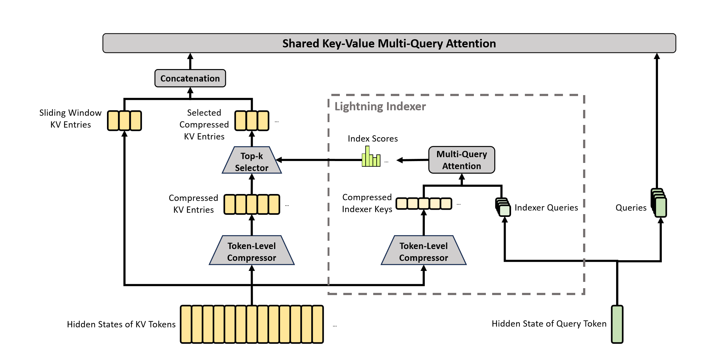
Figure 3 里有三条流:
- Sliding Window KV Entries: 最近一小段 token 不压缩,直接参加 attention,用来保留局部细粒度信息。
- Compressed KV Entries: 历史 KV 先由 token-level compressor 压缩,再由 top-k selector 选一部分进入 attention。
- Lightning Indexer: 不直接输出 hidden state,只给 compressed KV entries 打分并选择 top-k。
一句话概括:CSA 不是把所有历史 token 都扔进 attention,而是先把每 $m$ 个 KV 压成一个 entry,再让每个 query 只 attend 到 top-k 个 compressed entries,同时额外保留最近 sliding window 的原始 KV。
6.1 Compressed Key-Value Entries
论文从输入 hidden states 开始:
\[H\in\mathbb{R}^{n\times d}\]其中 $n$ 是 sequence length,$d$ 是 hidden size。CSA 先计算两组 KV entries:
\[C^a,C^b\in\mathbb{R}^{n\times c}\]以及两组对应的 compression weights:
\[Z^a,Z^b\in\mathbb{R}^{n\times c}\]这里 $c$ 是 head dimension。更细地说:
- $C^a,C^b$ 是两套 original KV entries,后面会被加权压缩成 compressed KV entries。
- $Z^a,Z^b$ 不是最终 KV,而是和 $C^a,C^b$ 同形状的 compression logits / weights,用来决定窗口内不同 token 的压缩权重。
- 上标 $a,b$ 表示两组 interleaved / overlapping series,不是 attention head 编号。
对第 $i$ 个 compressed entry,论文把两个长度为 $m$ 的连续片段拼起来看:
\[\begin{aligned} C^b_{m(i-1):mi-1} &\in \mathbb{R}^{m\times c} \\ C^a_{mi:m(i+1)-1} &\in \mathbb{R}^{m\times c} \end{aligned}\]也就是说,$b$ 组的 $m$ 个 token 在前,$a$ 组的 $m$ 个 token 紧接在后。对 $C_i^{\mathrm{Comp}}$ 来说,它实际聚合了一个长度为 $2m$ 的邻域信息:
\[\left[ m(i-1),\; m(i+1)-1 \right]\]但输出仍然只有一个 compressed entry。
论文公式可以理解成两步。第一步,先在这 $2m$ 个位置上做 compression softmax:
\[\begin{aligned} \left[ S^a_{mi:m(i+1)-1}; S^b_{m(i-1):mi-1} \right] &= \mathrm{Softmax}_{\mathrm{row}} \left( \left[ Z^a_{mi:m(i+1)-1}; Z^b_{m(i-1):mi-1} \right] + \left[ b^a; b^b \right] \right) \end{aligned}\]其中:
- $S^a,S^b$ 是真正用于加权求和的 compression scores。
- $b^a,b^b\in\mathbb{R}^{m\times c}$ 是 learnable compression biases。
- $\mathrm{Softmax}_{\mathrm{row}}$ 表示沿 token/window 这一维归一化;对每个 head dimension,都在这 $2m$ 个候选 token 上分配权重。
第二步,用这些 scores 加权两组 KV entries:
\[\begin{aligned} C_i^{\mathrm{Comp}} &= \sum_{j=mi}^{m(i+1)-1} S^a_j\odot C^a_j + \sum_{j=m(i-1)}^{mi-1} S^b_j\odot C^b_j \end{aligned}\]其中 $\odot$ 是逐维乘法。因为每个 $C^a_j,C^b_j\in\mathbb{R}^{c}$,所以:
\[C_i^{\mathrm{Comp}}\in\mathbb{R}^{c}\]现在再回答“为什么有 overlap 还能压缩到 $1/m$”:因为输出 index 还是按 $i$ 走,每 $m$ 个 token 产生一个 $C_i^{\mathrm{Comp}}$。overlap 只改变一个 compressed entry 聚合时能看的范围,让它看见 $2m$ 个 token;它不改变输出 stride。于是 entries 数量仍然约为:
\[\frac{n}{m}\]所以压缩率仍然约为:
\[\frac{1}{m}\]一个更具体的例子:如果 $m=4$,那么 $C_i^{\mathrm{Comp}}$ 聚合的是前一个 block 的 4 个 token 和当前 block 的 4 个 token,一共 8 个 token 的信息;但它仍然只输出 1 个 $c$ 维 compressed KV entry。
边界条件也要注意:当 $i=0$ 时,$m(i-1):mi-1$ 这一段不存在。论文说这个 undefined 的 segment 会被忽略。实现上通常可以理解为 mask 掉非法位置,让 softmax 不给这些位置分配权重。
6.2 Lightning Indexer for Sparse Selection
压缩后的 $C^{\mathrm{Comp}}$ 仍然很多。例如 1M context、$m=4$ 时,远程 compressed entries 仍然是十万级。CSA 不会把所有 compressed entries 都送进 core attention,而是借用 DSA strategy,先用一个轻量 indexer 做 top-k selection。
这一节最容易混淆的点是:Indexer 不是最终 attention。它只负责从 $C^{\mathrm{Comp}}$ 中选出 $C_t^{\mathrm{SprsComp}}$,然后 core attention 再读取这些 selected entries。
6.2.1 Indexer keys
论文先对历史 hidden states 做一次和 $C^{\mathrm{Comp}}$ 类似的压缩,但这里压缩出来的是 indexer keys,而不是最终参与 attention 的 KV entries:
\[K^{\mathrm{IComp}}\in \mathbb{R}^{\frac{n}{m}\times c^I}\]其中 $c^I$ 是 indexer head dimension。第 $s$ 个 compressed block 的 indexer key 记作 $K_s^{\mathrm{IComp}}\in \mathbb{R}^{c^I}$。可以把它理解成每个 compressed block 的“检索向量”。真正被选中的内容仍然来自 $C_s^{\mathrm{Comp}}$。
6.2.2 Indexer queries
对 query token $t$,论文从它的 hidden state $h_t$ 生成 indexer queries。第一步是 down-projection:
\[c_t^Q = h_t \cdot W^{DQ}\]然后再 up-projection 成 $n^{I}_{h}$ 个 indexer query heads:
\[\begin{aligned} \left[q^{I}_{t,1};q^{I}_{t,2};\ldots;q^{I}_{t,n^{I}_{h}}\right] &= q_t^I = c_t^Q \cdot W^{IUQ} \end{aligned}\]维度对应关系如下:
- $h_t\in \mathbb{R}^{d}$:query token $t$ 的输入 hidden state。
- $c_t^Q\in \mathbb{R}^{d_c}$:query compressed latent vector。
- $W^{DQ}\in \mathbb{R}^{d\times d_c}$:indexer query 的 down-projection matrix。
- $W^{IUQ}\in \mathbb{R}^{d_c\times c^I n^{I}_{h}}$:indexer query 的 up-projection matrix。
- $q^{I}_{t,h}\in \mathbb{R}^{c^I}$:第 $h$ 个 indexer query head。
这里的“先 down 再 up”不是为了还原原始 hidden state,而是为了用较低秩的 $c_t^Q$ 生成多头 indexer queries。后面的 core attention query 也会复用这个 $c_t^Q$。
6.2.3 DSA index score
接下来,论文给每个 indexer query head 一个 query-dependent weight:
\[\begin{aligned} \left[w^{I}_{t,1};w^{I}_{t,2};\ldots;w^{I}_{t,n^{I}_{h}}\right] &= w_t^I = h_t \cdot W^w \end{aligned}\]其中 $W^w\in \mathbb{R}^{d\times n^{I}{h}}$,$w^{I}{t,h}\in \mathbb{R}$。然后计算 query token $t$ 对 preceding compressed block $s$ 的 index score:
\[\begin{aligned} I_{t,s} &= \sum_{h=1}^{n^{I}_{h}} w^{I}_{t,h}\cdot \mathrm{ReLU}\left(q^{I}_{t,h}\cdot K_s^{\mathrm{IComp}}\right) \end{aligned}\]这里 $s<\left\lfloor t/m\right\rfloor$,表示只从 query token 之前的 compressed blocks 中选。这个公式可以拆成三层看:
- $q^{I}_{t,h}\cdot K_s^{\mathrm{IComp}}$:第 $h$ 个 indexer head 对 block $s$ 的相似度。
- $\mathrm{ReLU}(\cdot)$:只保留正相关的 block。
- $w^{I}_{t,h}$:让不同 query token 动态决定哪些 indexer heads 更重要。
得到所有 $I_{t,:}$ 之后,用 top-k selector 保留对应的 compressed KV entries:
\[\begin{aligned} C_t^{\mathrm{SprsComp}} &= \left\{ C_s^{\mathrm{Comp}} \mid I_{t,s}\in \mathrm{Top}\text{-}k\left(I_{t,:}\right) \right\} \end{aligned}\]注意 top-k 选的是 $C_s^{\mathrm{Comp}}$,不是 $K_s^{\mathrm{IComp}}$。$K^{\mathrm{IComp}}$ 只负责打分,$C^{\mathrm{Comp}}$ 才是后面 core attention 的 key/value 来源。
6.2.4 伪代码
def lightning_indexer(h_t, K_IComp, C_Comp, top_k):
    # Eq. (13): low-rank latent for the query token
    c_Q_t = h_t @ W_DQ

    # Eq. (14): n_h^I indexer query heads, each with dimension c^I
    q_I_t = (c_Q_t @ W_IUQ).reshape(n_h_I, c_I)

    # Eq. (15): query-dependent weights for indexer heads
    w_I_t = h_t @ W_w

    scores = []
    for s, K_s_IComp in enumerate(K_IComp):
        # Eq. (16): DSA-style sparse selection score
        score = 0.0
        for h in range(n_h_I):
            score += w_I_t[h] * relu(dot(q_I_t[h], K_s_IComp))
        scores.append(score)

    selected_blocks = topk(scores, k=top_k)

    # Eq. (17): selected compressed KV entries for core attention
    return [C_Comp[s] for s in selected_blocks]
6.3 Shared Key-Value Multi-Query Attention
选出 $C_t^{\mathrm{SprsComp}}$ 之后,CSA 才进入真正的 core attention。论文这里采用 Multi-Query Attention 的形式:每个 compressed KV entry 同时作为 key 和 value,而 query 有 $n_h$ 个 heads。
先从前面已经得到的 $c_t^Q$ 生成 core attention queries:
\[\begin{aligned} \left[q_{t,1};q_{t,2};\ldots;q_{t,n_h}\right] &= q_t = c_t^Q \cdot W^{UQ} \end{aligned}\]其中 $n_h$ 是 query heads 数量,$W^{UQ}\in \mathbb{R}^{d_c\times c n_h}$,每个 $q_{t,i}\in \mathbb{R}^{c}$。论文特别说明:这里的 latent query vector $c_t^Q$ 和 indexer queries 使用的是同一个 $c_t^Q$。
然后对每个 query head 做 core attention:
\[\begin{aligned} o_{t,i} &= \mathrm{CoreAttn} \left( \mathrm{query}=q_{t,i}, \mathrm{key}=C_t^{\mathrm{SprsComp}}, \mathrm{value}=C_t^{\mathrm{SprsComp}} \right) \end{aligned}\]其中 $o_{t,i}\in \mathbb{R}^{c}$。Figure 3 里还会把 selected compressed KV entries 与 sliding window KV entries concat 后送入 shared key-value MQA;公式 (19) 写的是 sparse compressed branch 的核心形式。保留 sliding window KV 的目的,是让最近 token 的 fine-grained dependencies 不完全依赖压缩表示。
6.4 Grouped Output Projection
Core attention 之后会得到 $n_h$ 个 head outputs:
\[\begin{aligned} \left[o_{t,1};o_{t,2};\ldots;o_{t,n_h}\right] &= o_t \in \mathbb{R}^{c n_h} \end{aligned}\]如果直接把 $o_t\in \mathbb{R}^{c n_h}$ 投影回 $d$ 维 hidden state,计算量大约是:
\[\mathcal{O}\left(c n_h d\right)\]论文说 DeepSeek-V4 中 $c n_h$ 很大,所以直接做 output projection 会很贵。Grouped Output Projection 的做法是先把 $n_h$ 个 outputs 分成 $g$ 组。第 $i$ 组输出满足:
\[o^G_{t,i}\in \mathbb{R}^{c\frac{n_h}{g}}\]每一组先投影到一个更小的 intermediate output:
\[o^{G'}_{t,i}\in \mathbb{R}^{d_g}, \qquad d_g < c\frac{n_h}{g}\]最后再把所有组的 intermediate outputs 拼接:
\[\begin{aligned} \left[o^{G'}_{t,1};o^{G'}_{t,2};\ldots;o^{G'}_{t,g}\right] &\in \mathbb{R}^{d_g g} \end{aligned}\]并投影成最终 attention output:
\[\hat{o}_t\in \mathbb{R}^{d}\]直观计算量可以写成两段:
\[\mathcal{O}\left(c n_h d_g\right) + \mathcal{O}\left(g d_g d\right)\]因为 $d_g < c\frac{n_h}{g}$,第一段相当于先在每组内部做 bottleneck compression;第二段再做跨组混合。它比直接 $c n_h\rightarrow d$ 更省的核心原因是:不再让一个巨大矩阵同时处理所有 heads 到 $d$ 维,而是先把每组 head outputs 压到较小的 $d_g$。
6.5 Attention Sink
论文在 CSA / HCA 的 core attention 里还用了 Attention Sink。这一节的 $h$ 是 attention head 的编号,不是 mHC 里的 $n_{\mathrm{hc}}$。
普通 attention 会把一个 head 的全部权重都分给真实 token / compressed block:
\[\sum_j s_{h,i,j}=1\]但在长上下文压缩场景里,有些 compressed block 对当前 query 可能没用。如果没有 sink,这个 head 还是必须把 100% 概率质量硬分给它们,可能引入噪声。
论文的做法是给每个 attention head 加一个可学习的 sink logit $z’_h$,并把 $\exp(z’_h)$ 加进 softmax 分母:
\[\begin{aligned} s_{h,i,j} &= \frac{\exp(z_{h,i,j})} {\sum_k\exp(z_{h,i,k})+\exp(z'_h)} \end{aligned}\]其中:
- $z_{h,i,j}$:第 $h$ 个 attention head 中,第 $i$ 个 query token 对第 $j$ 个 preceding token / compressed block 的 attention logit。
- $s_{h,i,j}$:对应的 attention score。
- $z’_h$:第 $h$ 个 attention head 的 learnable sink logit。
这样真实 KV 上的总 attention mass 变成:
\[\begin{aligned} \sum_j s_{h,i,j} &= \frac{\sum_j\exp(z_{h,i,j})} {\sum_k\exp(z_{h,i,k})+\exp(z'_h)} \le 1 \end{aligned}\]剩下的概率质量被 sink 吃掉,不参与 value 聚合。直觉上,这允许某个 head 表达“这次这条 attention branch 没什么可看的”,而不是强迫它在一堆低相关 compressed entries 里硬选。
6.6 Hugging Face 对应代码
HF / 官方 inference 里的 CSA 关键路径可以分成两块:Compressor 负责生成 compressed entries,Indexer 负责从这些 entries 中选 top-k。下面是保留变量含义后的删减版。
# Compressor: C / Z / compression bias
coff = 1 + overlap
ape = Parameter([compress_ratio, coff * head_dim])
wkv = Linear(dim, coff * head_dim)
wgate = Linear(dim, coff * head_dim)

kv = wkv(hidden_states)       # corresponds to C entries
score = wgate(hidden_states)  # corresponds to Z weights

kv = kv.unflatten(1, (-1, compress_ratio))
score = score.unflatten(1, (-1, compress_ratio)) + ape

if overlap:
    kv = overlap_transform(kv, value=0)
    score = overlap_transform(score, value=-inf)

kv = (kv * score.softmax(dim=2)).sum(dim=2)
kv = norm(kv)
当 overlap=True 时,overlap_transform 对应论文里的 $C^b_{m(i-1):mi-1}$ 和 $C^a_{mi:m(i+1)-1}$ 拼接;当 compress_ratio=4 时,这就是 CSA 的 compressed KV 生成方式。
# Indexer: Eq. (13)-(17)
c_Q_t = h_t @ W_DQ
q_I_t = (c_Q_t @ W_IUQ).reshape(n_h_I, c_I)
w_I_t = h_t @ W_w

raw = q_I_t @ K_IComp.transpose(-1, -2)
scores = (relu(raw) * w_I_t[:, None]).sum(dim=0)

selected_indices = topk(scores, k=index_topk)
C_t_SprsComp = gather(C_Comp, selected_indices)
最后 Attention Sink 对应的是每个 head 一个 learnable sink logit。它不会产生新的 value,只改 softmax 分母:
denom = exp(attn_logits).sum(dim=-1, keepdim=True) + exp(sink_logits)
attn_scores = exp(attn_logits) / denom
7. HCA: Heavily Compressed Attention
HCA = Heavily Compressed Attention。
相比 CSA,HCA 更直接:
- 不做 overlap。
- 不做 indexer。
- 用更大的压缩窗口,例如 $m’=128$。
- 每 $m’$ 个 token 压成一个 compressed entry。
对应公式更接近:
\[\begin{aligned} C^{\mathrm{HCA}}_i &= \sum_{j=0}^{m'-1} \mathrm{softmax}(Z_{i,j}+B_j)\, C_{i,j} \end{aligned}\]HCA 的定位不是“精确找远程细节”,而是“用很小代价保存远程上下文的粗粒度记忆”。
| Layer type | Compress rate | Overlap | Indexer | KV 形态 |
|---|---|---|---|---|
| Sliding window attention | 0 | No | No | 最近窗口原始 KV |
| CSA | 4 | Yes | Yes | 原始窗口 KV + selected compressed KV |
| HCA | 128 | No | No | 原始窗口 KV + 全部 heavily compressed KV |
官方 inference 默认 compress_ratios 类似:
(0, 0, 4, 128, 4, 128, 4, 0)
这说明不同层混合使用无压缩、CSA 和 HCA。这个设计挺合理:不是所有层都需要同一种长程记忆,一些层负责精确,一些层负责便宜地扫远处。
HCA 在代码上仍然复用 Compressor,关键差异是压缩率更大、不开 overlap、也不走 indexer:
compress_ratio = 128
overlap = False

kv = wkv(hidden_states)
score = wgate(hidden_states) + ape

kv = kv.unflatten(1, (-1, compress_ratio))
score = score.unflatten(1, (-1, compress_ratio))

kv = (kv * score.softmax(dim=2)).sum(dim=2)
kv = norm(kv)
所以 HCA 的代码路径比 CSA 少两件事:没有 overlap_transform,也没有 Indexer -> topk -> gather(C_Comp)。
8. Muon Optimizer
DeepSeek-V4 的更新不只在 attention 和 MoE 上,也包括训练优化器。模型卡和论文摘要里都把 Muon optimizer 列为训练侧改动:它服务于更快收敛和更稳定的大规模预训练,而不是推理时的网络结构。
Muon 通常展开为 Momentum Orthogonalized by Newton-Schulz。它的核心不是像 AdamW 那样给每个参数做逐元素自适应缩放,而是把二维权重矩阵的梯度更新看成一个矩阵,再对 momentum update 做近似正交化。
可以用下面的抽象公式理解:
\[\begin{aligned} G_t &= \nabla_W \mathcal{L}(W_t) \\ M_t &= \mu M_{t-1}+G_t \\ \hat{M}_t &= \mathrm{NewtonSchulz}(M_t) \\ W_{t+1} &= W_t-\eta \hat{M}_t \end{aligned}\]其中:
- $G_t$:当前 step 对权重矩阵 $W_t$ 的梯度。
- $M_t$:带 momentum 的更新方向。
- $\mathrm{NewtonSchulz}(\cdot)$:用 Newton-Schulz iteration 做近似正交化,让更新方向在矩阵谱上更均衡。
- $\hat{M}_t$:正交化后的更新方向。
直觉上,Muon 希望避免某些奇异方向被更新得过强、另一些方向几乎不动。对大模型里的线性层矩阵来说,这种矩阵级更新比逐元素缩放更贴近“层”的结构。
一个很粗略的 Newton-Schulz 伪代码是:
G = grad(W)
M = momentum * M + G

X = normalize(M)
for _ in range(num_ns_steps):
    A = X @ X.T
    X = a * X + b * (A @ X) + c * (A @ A @ X)

W = W - lr * X
这段伪代码只表达机制,不等价于 DeepSeek-V4 的完整训练实现。实际训练里还要处理参数分组、混合精度、分布式并行和不同参数类型的 optimizer 分配。对这篇笔记来说,最重要的结论是:Muon 是训练稳定性和收敛速度的优化,不改变推理时的 forward graph;CSA、HCA、mHC、MoE router 才是模型结构里的主要变化。
9. MoE Runtime Optimization
DeepSeek-V4 论文里还有一个容易被忽略但很重要的系统优化:Fine-Grained Communication-Computation Overlap in Expert Parallelism。它不是改 MoE 的数学定义,也不是改变 router 选专家的规则,而是在 expert parallelism 下重新安排 MoE 层的执行顺序。
论文把一个 MoE 层拆成通信和计算交替出现的五段:
Dispatch All-to-All
-> Linear-1 GEMM
-> SwiGLU + FP8 Cast
-> Linear-2 GEMM
-> Combine All-to-All
其中 Linear-1 和 Linear-2 是 expert FFN 内部天然存在的两个 GEMM,不是额外引入的新结构。如果 expert 使用 SwiGLU,那么 Linear-1 通常同时产生 gate/up 两路中间表示,SwiGLU + FP8 Cast 把中间激活重新量化后交给 Linear-2。
9.1 wave 到底是什么
DeepSeek-V4 的关键做法是把 local experts 进一步切成多个 expert waves。一个 wave 不是 token chunk,也不是某个 expert 的一个 GEMM tile,而是一小批 experts 及其对应的 routed tokens。
论文里的调度逻辑可以理解成:
wave 0 的 experts 完成 dispatch -> 立刻开始 Linear-1 / Act / Linear-2
wave 1 的 experts 仍在接收 token -> 通信继续推进
wave -1 的 experts 已经算完 -> output 立刻 combine 回原 rank
进入稳态后,同一时刻可以同时发生三件事:
combine previous wave | compute current wave | dispatch next wave
这就是它和普通 EP overlap 的区别。普通做法经常是“整层 dispatch 完成后再算,整层算完后再 combine”;DeepSeek-V4 让每个 wave 准备好就进入计算,不等其他 experts。这样可以减少 long-tail expert 或小 batch 场景下的空转,论文特别提到 RL rollout 和 high-speed agent serving 这类 latency-sensitive 场景会受益。
9.2 为什么通信能被盖住
论文给出的判断不是“带宽越高越好”,而是看计算通信比:
\[\frac{C}{B}\leq \frac{V_{\mathrm{comp}}}{V_{\mathrm{comm}}}\]其中 $C$ 是设备峰值计算能力,$B$ 是互联带宽,$V_{\mathrm{comp}}$ 是 MoE 计算量,$V_{\mathrm{comm}}$ 是 MoE 通信量。
对 DeepSeek-V4-Pro,一个 token-expert pair 的 SwiGLU expert 大约需要:
\[V_{\mathrm{comp}}\approx 6hd\]这里的 $h$ 是 hidden size,$d$ 是 intermediate hidden size。三项来自 gate projection、up projection、down projection。通信量约为:
\[V_{\mathrm{comm}}\approx 3h\]这里对应 FP8 dispatch 和 BF16 combine。因此:
\[\frac{V_{\mathrm{comp}}}{V_{\mathrm{comm}}}\approx 2d\]当 $d=3072$ 时,阈值约为:
\[2d=6144\ \mathrm{FLOPs/Byte}\]含义是:如果硬件的 $C/B$ 不超过这个比例,那么通信理论上可以被 expert GEMM 覆盖;继续堆更多互联带宽的收益会下降,反而要保证计算、显存和网络能同时高负载运行。
9.3 公开代码能看到什么
论文说已经开源 CUDA-based mega-kernel MegaMoE2,位置在 DeepGEMM。DeepGEMM PR #304 对这个 kernel 的描述很直接:它把 dispatch / linear 1 / SwiGLU / linear 2 / combine 融合进一个 mega-kernel,并重叠 NVLink communication 和 tensor core computation。
公开测试文件 tests/test_mega_moe.py 能看到两个路径的对照:
# fused path
buffer = get_symm_buffer_for_mega_moe(...)
transformed_l1_weights, transformed_l2_weights = transform_weights_for_mega_moe(...)
fp8_fp4_mega_moe(
    y,
    transformed_l1_weights,
    transformed_l2_weights,
    buffer,
    cumulative_local_expert_recv_stats=...,
)

# legacy baseline
recv_x, handle = ep_buffer.dispatch(...)
l1_y = grouped_fp8_fp4_gemm(recv_x, l1_weights, ...)
l1_y = swiglu_and_cast(l1_y, topk_weights, ...)
l2_y = grouped_fp8_fp4_gemm(l1_y, l2_weights, ...)
y = ep_buffer.combine(l2_y, handle=handle)
这段对照很有用:它说明 MegaMoE2 不是单独优化某一个 GEMM,而是把 EP dispatch、两次 expert GEMM、SwiGLU/cast、combine 都放进同一个 fused runtime 里处理。Python API 层没有暴露 num_waves 这种模型超参数;wave 更像 kernel 内部的调度粒度,由 routed token metadata、local expert receive stats、symmetric buffer 和 transformed expert weights 共同驱动。
PR #316 的 benchmark 也和论文说法一致:在 EP8 下,DeepSeek-V4-Flash 使用 256 experts、top-k=6、hidden size 4096、intermediate size 2048;DeepSeek-V4-Pro 使用 384 experts、top-k=6、hidden size 7168、intermediate size 3072。不同 batch size 下相对 legacy baseline 大约有 1.50x 到 1.96x 的加速,其中小 batch latency 场景收益更明显。
9.4 论文给硬件和 kernel 的几个观察
DeepSeek-V4 这节最后还有几个系统侧观察,值得单独记下来:
- 不是无限堆带宽。 当 $C/B$ 已经低于 $2d$ 这个阈值后,继续增加互联带宽的边际收益下降;更重要的是让 compute、memory、network 同时保持高负载。
- power budget 会变成瓶颈。 极端融合会让 Tensor Core、HBM、NVLink 同时繁忙,功耗墙可能比单看 FLOPs 或带宽更早出现。
- dispatch 采用 pull-based 思路。 论文说 dispatch 阶段由每个 GPU 主动读取远端 activations,避免 fine-grained push 带来的高通知延迟;如果未来硬件有更低延迟的跨 GPU signaling,push 才会更自然。
- SwiGLU 本身也可能阻塞 pipeline。 因为 SwiGLU 有指数和除法相关开销,论文建议未来可以考虑更低成本的 element-wise activation,减少 post-GEMM 处理对 GEMM pipeline 的打断。
这类优化和 MiniMax-01、Comet、FlashMoE 都有关,但粒度不同:MiniMax-01 更偏 token group / process group 级 overlap;Comet 更偏 shared tensor / GEMM tile 级重排;FlashMoE 更激进,把 MoE 执行放进 persistent kernel 里调度;DeepSeek-V4 则采用 expert-wave pipeline 来服务自己的大规模 MoE 推理与训练系统。
更完整的比较我单独整理在这里:MoE 优化的探索。
10. 总结表
| 模块 | 解决的问题 | 核心机制 | 代价 | 源码入口 |
|---|---|---|---|---|
| MTP | next-token 信号太局部 | 预测未来多个 token | 额外 MTP block/head 计算 | MTPBlock |
| MoE Router | MoE routing scores 需要平滑非负,并选择 experts | softplus/sqrtsoftplus scores + top-k/hash route | selection 和 weighting 逻辑更复杂 | Gate / DeepseekV4TopKRouter |
| Hash Route | 早期层动态路由成本和波动 | token id 查表得到 experts | 上下文自适应弱一些 | tid2eid / DeepseekV4HashRouter |
| MoE Runtime Optimization | expert parallelism 下通信阻塞计算 | expert waves + MegaMoE2 fused runtime | kernel 调度和实现复杂度更高 | DeepGEMM fp8_fp4_mega_moe |
| mHC | 深层 residual 信号传播 | 多 stream + Sinkhorn mixing | 小矩阵归一化开销 | DeepseekV4HyperConnection |
| CSA | 远程上下文太长 | 近邻原始 KV + $C_t^{\mathrm{SprsComp}}$ + shared KV MQA | 需要 compressor 和 indexer | DeepseekV4CSACompressor |
| HCA | 更便宜的远程记忆 | 大窗口压缩,无 indexer | 细节损失更大 | DeepseekV4HCACompressor |
| Attention Sink | compressed KV 无关时不应强制分配满权重 | 分母加入 learnable sink logit | 每个 head 多一个 sink 参数 | attention score computation |
| Lightning Indexer | compressed entries 仍然太多 | $K^{\mathrm{IComp}}$ 与 $q^I_t$ 计算 $I_{t,s}$ 后 top-k | 可能漏选远程关键信息 | Indexer / DeepseekV4Indexer |
| Grouped Output Projection | $c n_h\rightarrow d$ 直接投影太贵 | 先按 $g$ 组压到 $d_g$,再投影到 $d$ | 增加 per-group bottleneck | attention output projection |
| Muon Optimizer | 大规模预训练收敛和稳定性 | momentum update + Newton-Schulz 近似正交化 | 训练侧额外 optimizer 计算 | training optimizer |
11. 源码与资料入口
- DeepSeek-V4 Technical Report: DeepSeek_V4.pdf
- DeepSeek-V4-Pro Model Card: deepseek-ai/DeepSeek-V4-Pro
- Official inference code: inference/model.py
- Official encoding code: encoding/encoding_dsv4.py
- DeepGEMM MegaMoE2 PR: deepseek-ai/DeepGEMM#304
- DeepGEMM MegaMoE2 Benchmark PR: deepseek-ai/DeepGEMM#316
- Transformers implementation: modeling_deepseek_v4.py
- Transformers config: configuration_deepseek_v4.py
- DeepSeek-V3 Technical Report, for MTP background: hf.co/papers/2412.19437
- mHC-lite discussion: hf.co/papers/2601.05732
- Sparse indexer related work: IndexCache, HISA
12. 最后的一句话理解
DeepSeek-V4 的主线不是“又把模型做大了”。它更像是在问一个工程问题:当上下文来到 1M tokens,模型到底应该怎样保存、压缩、索引和读取历史信息?
CSA、HCA、Lightning Indexer 解决的是 长上下文的读写成本;mHC 解决的是 深层网络里的信息传播稳定性;MTP、router 和 Muon 则分别服务于 训练信号密度、sparse computation 与预训练优化。把这些合起来,DeepSeek-V4 才有了 1M context 下还能工作的结构基础。